


What if your risk number ignored all the good days?
That’s what downside deviation does: it measures only the returns that fall below a chosen target (your minimum acceptable return).
If you care more about shortfalls than upside noise, this is the right tool.
In this post I will show you a clear, step-by-step way to measure downside deviation, pick the right denominator, run the math in Excel, annualize the result, and use it in performance metrics like the Sortino ratio.
You’ll finish knowing exactly how often and how badly your portfolio misses its goal.
Core Methodology for Measuring Downside Deviation Clearly and Accurately

1. Choose your target return (B) — You need to pick the minimum acceptable return (MAR). Could be 0%, your hurdle rate, or a benchmark threshold. For example: “Before settling on 5% as my MAR, I checked if that return matched my retirement income goal.”
2. Collect your return series — Gather periodic returns (monthly, quarterly, or annual) in decimal form. So 2% becomes 0.02, and a 3% loss becomes −0.03.
3. Calculate each deviation — For every return (Xi), subtract your target: Xi − B. If it’s positive or zero, ignore it. If it’s negative, you’ll use it.
4. Square each negative deviation — Take every shortfall from step 3 and square it: (Xi − B)². Squaring gets rid of the negative sign and makes larger shortfalls count more.
5. Sum the squared deviations — Add up all the squared shortfalls you kept in step 4. Returns that met or beat your target don’t enter the calculation.
6. Divide by your chosen denominator — You can divide by total observations (n), observations below target, or n − 1. It depends on whether you’re computing population or sample downside deviation.
7. Take the square root — Final downside deviation is the square root of the result from step 6, expressed in the same units as your returns (usually %).
Downside deviation measures volatility of returns that fall below a target return (B). It focuses only on losses or shortfalls. Gains? Totally ignored. This makes it a better fit for investors who worry more about underperformance than upside volatility.
The core formula (population form) is: s_Target = sqrt( Σ(Xi − B)² / n ). Only returns below B enter the sum. Semi‑variance is the average squared deviation below the target. Semi‑deviation is the square root of semi‑variance and is identical to downside deviation when the target equals your chosen threshold. Target semi‑deviation and target downside deviation? Same thing, different labels.
A downside deviation of 5% means returns below your target swung by about 5 percentage points on average. Lower values mean tighter clustering around or above the target. Higher values signal frequent or severe shortfalls.
Understanding the Downside Deviation Formula and Variance Logic

The denominator you choose changes the size of your downside deviation. Divide by total observations (n) when you want to penalize all periods equally, even the ones that met your target. Divide by the count of below‑target returns when you want a conditional measure reflecting only the periods of shortfall. Divide by n − 1 if you’re computing a sample statistic and want to correct for bias.
Each choice answers a different question. Using n treats every observation as part of the risk picture. Using the count of downside observations isolates average shortfall severity. Using n − 1 is common in academic settings and portfolio software that assume you’re estimating population risk from a sample. The difference is biggest when few returns fall below your target.
Use total observations (n) when you’re computing the Sortino ratio or another performance metric where consistency matters. Also when you want a stable denominator that doesn’t shift with market conditions, or you’re comparing multiple funds on equal footing.
Use the count of below‑target observations when you want to measure the average size of shortfalls conditional on a shortfall happening. You’re analyzing tail behavior in a regime‑switching market. Or you’re modeling downside‑only scenarios.
Required Inputs for Calculating Downside Deviation

You need a series of periodic returns covering a consistent time window. Monthly, quarterly, or annual returns all work, but the periodicity must match across your entire dataset. Express returns in decimal form (2% becomes 0.02, −3% becomes −0.03) to avoid multiplication errors.
Choose a target return (B) or minimum acceptable return (MAR). Could be zero, a hurdle rate, a benchmark index return, or the mean of your dataset. The choice depends on your investment objective. Managing against a 4% distribution requirement? Use 4%. Care about absolute losses? Use zero. State your choice explicitly when reporting results because the same return series will produce different downside deviations under different targets.
Step‑by‑Step Manual Calculation of Downside Deviation

The worked example uses annual returns from 2010 to 2020 and a target of 20%. Any return below 20% counts as a shortfall. Any return at or above 20% is ignored. The squared deviations sum to 2,961 percentage points, the denominator is 10 (eleven observations minus one for a sample correction), and the final downside deviation is 17.21%.
This shows how a few large negative deviations (2018 and 2019) dominate the sum even when most years meet or exceed the target. That’s exactly what downside deviation is designed to capture: the volatility of underperformance.
| Year | Return | Deviation from 20% | Squared Deviation |
|---|---|---|---|
| 2010 | 36% | — | — |
| 2011 | 29% | — | — |
| 2012 | 10% | −10% | 100 |
| 2013 | 52% | — | — |
| 2014 | 41% | — | — |
| 2015 | 16% | −4% | 16 |
| 2016 | 10% | −10% | 100 |
| 2017 | 23% | — | — |
| 2018 | −10% | −30% | 900 |
| 2019 | −19% | −39% | 1,521 |
| 2020 | 2% | −18% | 324 |
Using Excel to Measure Downside Deviation Efficiently

Excel can automate every step. Most common approach uses SUMPRODUCT to multiply each squared deviation by a condition checking whether the return is below the target. The formula divides the result by total observations or count of shortfalls, then takes the square root. Legacy Excel versions require Ctrl+Shift+Enter for array formulas. Modern Excel with dynamic arrays accepts them without special input.
Watch your cell references. Use absolute references ($B$1) for the target so the formula copies correctly. Make sure your return range and denominator function (COUNT or COUNTIF) cover the same cells. A mismatch creates silent errors that mess up your result.
- Divide by total observations (sample form): =SQRT(SUMPRODUCT((A2:A13-$B$1)^2*(A2:A13<$B$1))/(COUNT(A2:A13)-1))
- Divide by downside count: =SQRT(SUMPRODUCT((A2:A13-$B$1)^2*(A2:A13<$B$1))/COUNTIF(A2:A13,”<“&$B$1))
- Array formula variant (legacy Excel, Ctrl+Shift+Enter): =SQRT(SUM(IF(A2:A13<$B$1,(A2:A13-$B$1)^2,0))/(COUNT(A2:A13)-1))
- Using AVERAGE for population form: =SQRT(AVERAGE(IF(A2:A13<$B$1,(A2:A13-$B$1)^2)))
- Dynamic array modern Excel (no special entry): =SQRT(SUMPRODUCT((A2:A13-$B$1)^2*(A2:A13<$B$1))/COUNTA(A2:A13))
Annualizing and Interpreting Downside Deviation

If you compute downside deviation using monthly returns, multiply the result by the square root of 12 (3.4641) to annualize it. For daily returns (assuming 252 trading days), multiply by sqrt(252), which is 15.8745. For quarterly returns, multiply by sqrt(4), or 2.0. Annualization assumes returns are independent and identically distributed, so be cautious if your portfolio shows serial correlation or regime shifts.
A downside deviation of 17.21% (like in the 2010–2020 example with a 20% target) tells you that shortfalls swung by about 17 percentage points on average. If you’re managing against a hurdle rate, this number quantifies how volatile underperformance has been. Lower downside deviation means more stable returns around or above your threshold. Higher values warn that when the fund missed the target, it missed by a lot.
How Downside Deviation Compares with Standard Deviation and Semi‑Deviation
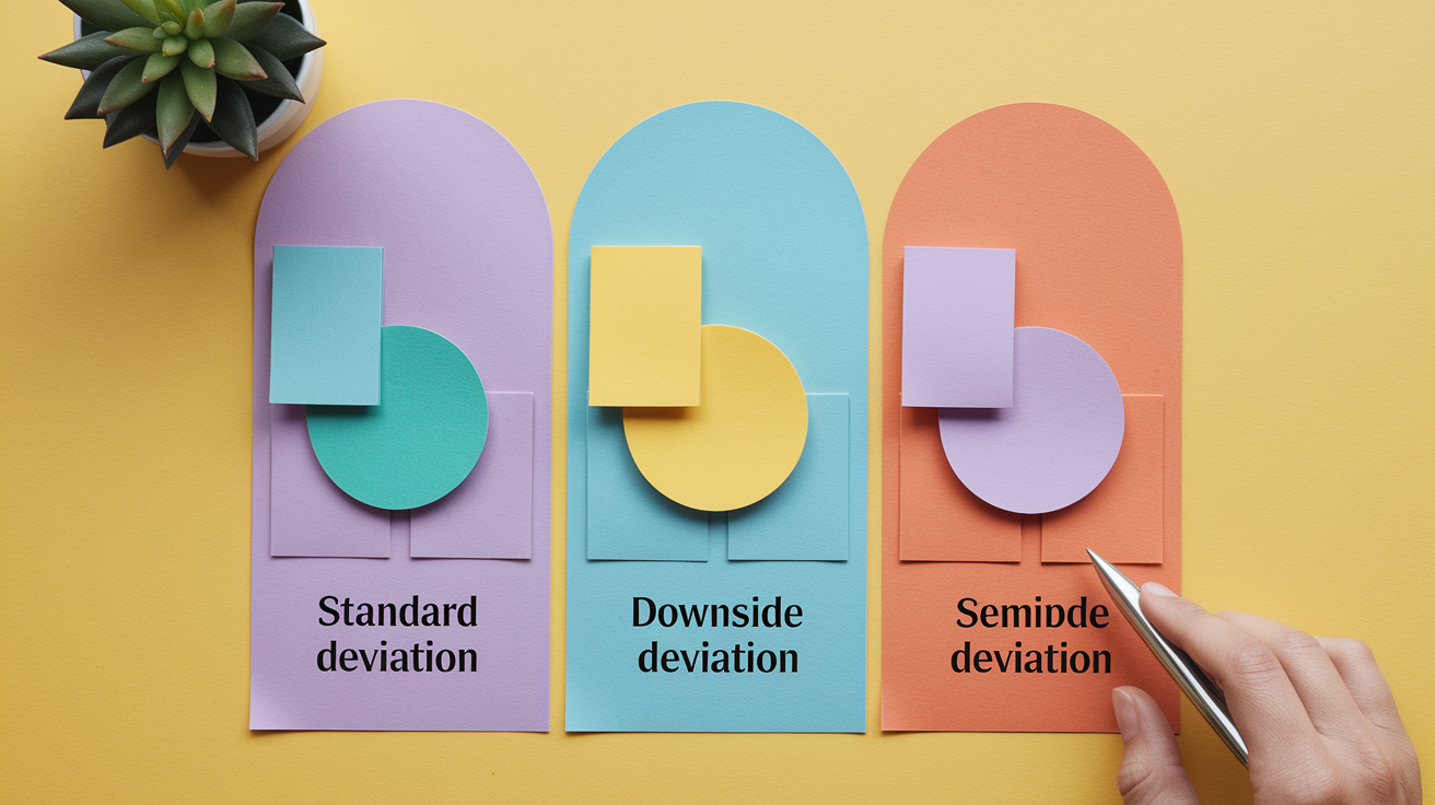
Standard deviation treats upside and downside volatility the same. A fund that swings 10% above and 10% below the mean gets the same standard deviation as one swinging only below. That symmetry works fine for normally distributed returns but misleads when returns are skewed. Downside deviation ignores positive deviations entirely and focuses only on losses.
Semi‑deviation measures volatility below the mean, not below a target you choose. If your average return is 8% but your hurdle is 5%, semi‑deviation will penalize returns between 5% and 8%, even though they meet your requirement. Downside deviation (target semi‑deviation) lets you set the threshold that matters to you.
Use standard deviation when you care about total variability and returns are roughly symmetric. Use semi‑deviation when you want to isolate downside relative to the fund’s own average. Use downside deviation when you have a specific loss threshold or minimum acceptable return and want to measure risk against that benchmark.
Applying Downside Deviation in Performance Metrics (Including Sortino Ratio)
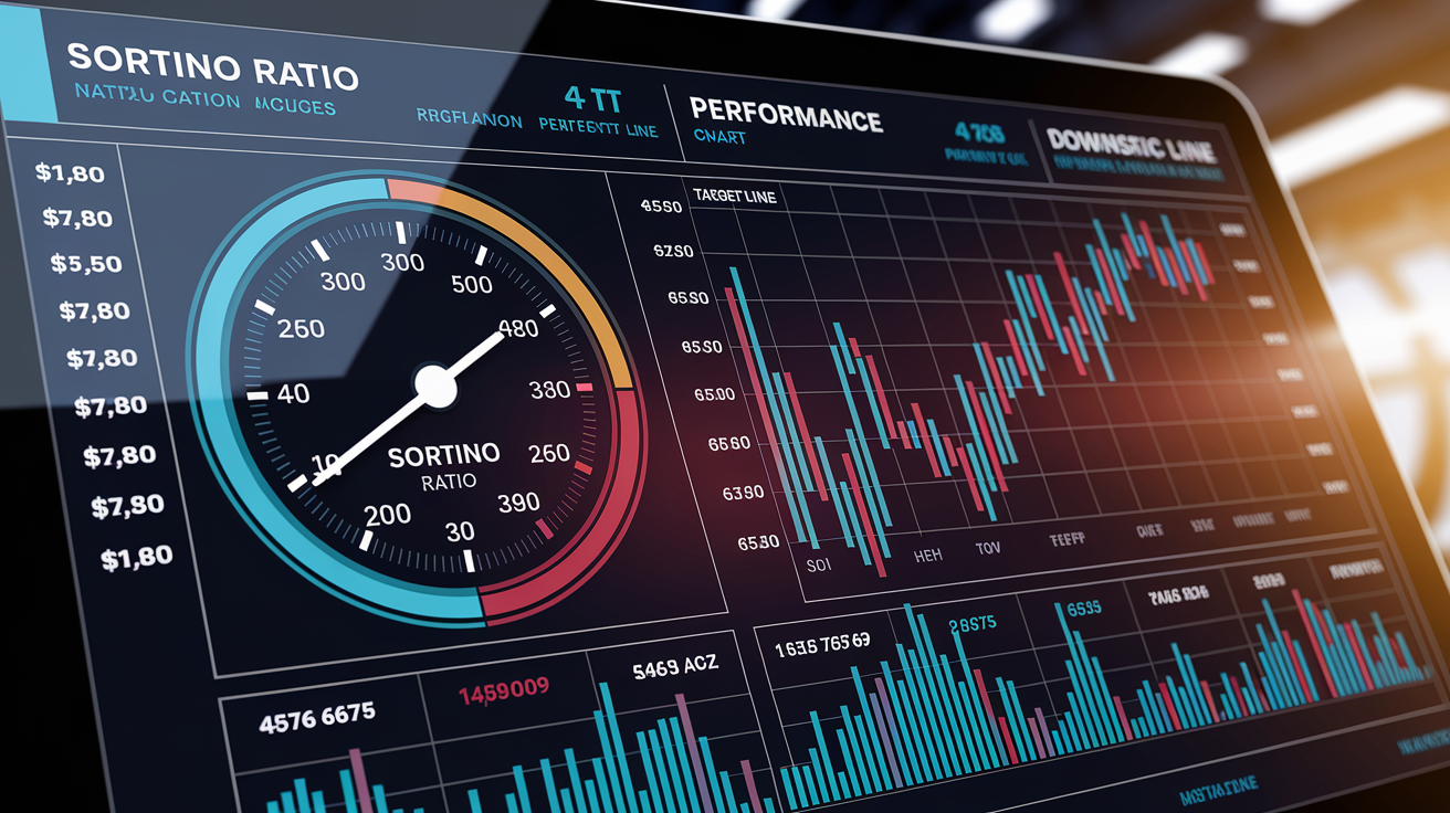
The Sortino ratio divides excess return by downside deviation instead of standard deviation. This rewards managers who deliver returns above the target without penalizing upside volatility. In the worked example, monthly downside deviation is 1.173%, annualized to 4.06%. Monthly return is 0.4583% (5.5% annual). The monthly Sortino ratio is 0.391. The annual Sortino is 1.355 (5.5% ÷ 4.06%). Both measure how much excess return you earned per unit of downside risk.
Downside deviation also appears in other performance tools. Some fund managers report it alongside standard deviation to show tail behavior. Risk‑budgeting frameworks use it to allocate capital based on downside rather than total volatility. Multi‑asset portfolios compare downside deviation across asset classes to identify which holdings contribute most to shortfall risk.
You can track downside deviation monthly to spot rising tail risk before it shows up in returns. Compare Sortino ratios across funds to identify managers who protect on the downside. Use downside deviation in scenario analysis to model losses under stress. Report both standard deviation and downside deviation to give a complete risk picture.
When to Use Downside Deviation vs VaR or CVaR

Value at Risk (VaR) estimates the loss threshold at a given confidence level (like 95% VaR means you expect to lose no more than that amount 95% of the time). It focuses on a single percentile and ignores the magnitude of losses beyond that point. Conditional Value at Risk (CVaR, also called Expected Shortfall) measures the average loss in the tail beyond the VaR cutoff, capturing both frequency and severity of extreme events.
Downside deviation summarizes all shortfalls below your target, not just tail events. If you have many small losses and a few large ones, downside deviation weights the large losses more (because it squares deviations) but still includes the small ones. VaR ignores everything above the percentile. CVaR averages only the tail. VaR computed under a normal distribution can understate risk when returns are skewed or heavy‑tailed. Modified Cornish‑Fisher VaR corrects for skewness and excess kurtosis.
Use downside deviation when you care about volatility of all below‑target returns, not just worst‑case scenarios. Or you’re computing a Sortino ratio or similar downside‑adjusted performance metric. Or you want a single number capturing both frequency and severity of underperformance.
Use VaR when regulations or internal policy require a percentile‑based loss limit, or you need a simple threshold for capital reserves or position sizing.
Use CVaR when tail severity matters more than overall downside volatility. Or you’re stress‑testing for catastrophic losses or managing portfolios with heavy tails.
Practical Challenges and Common Mistakes When Measuring Downside Deviation

Denominator ambiguity is the single biggest source of inconsistency. Software packages and academic papers use different conventions (n, n − 1, or count of downside observations) without always stating which. Always document your choice and verify that comparison data uses the same method. Choice of MAR also matters enormously: a 0% target and a 5% target will produce completely different numbers for the same return series.
Small samples amplify estimation error. Twelve monthly observations is the bare minimum. Thirty or more is better. Data expressed in percentages instead of decimals will produce errors 10,000 times too large if you forget to convert. Annualization assumes independent returns. If your portfolio shows momentum or mean reversion, the sqrt(n) multiplier overstates or understates true annual risk. Frequency mismatch (annual MAR, monthly returns) creates confusion unless you align everything to the same period before calculating.
State your denominator choice (n, n − 1, or downside count) explicitly in reports. Document the MAR and explain why you chose it. Use at least 24–36 observations to stabilize the estimate. Convert all returns to decimals before squaring and summing. Verify that your MAR, return frequency, and annualization multiplier all match.
Final Words
Start with the 7-step procedure: gather returns, pick your minimum acceptable return, keep only below-target values, square each shortfall, sum them, apply the chosen denominator, then take the square root. That sequence gets you the core number fast.
We also covered the formula idea, denominator choices, an Excel approach, the 17.21% example, annualizing, and how this fits into Sortino and other risk tools.
Use this guide to learn how to measure downside deviation and make steadier, simpler risk decisions going forward.
FAQ
Q: How do I calculate downside deviation?
A: You calculate downside deviation by isolating returns below a target, squaring those shortfalls, averaging the squared shortfalls, then taking the square root to express downside risk as a percent.
Q: What is the difference between standard deviation and downside deviation?
A: The difference is that standard deviation measures overall variability around the average, while downside deviation measures only returns below a chosen target, so it highlights the risk of losses investors care about.
Q: What is a 5% VaR?
A: A 5% VaR is the loss level expected to be exceeded only 5% of the time over a chosen period, estimating how bad losses can get in the worst 5 percent of outcomes.
Q: What does 0.5 standard deviation mean?
A: A 0.5 standard deviation means a value lies half as far from the mean as one full standard deviation, indicating relatively low variability and that outcomes tend to cluster nearer the average.