


What if the fund with the biggest returns is actually the worst deal for your money?
The Sharpe ratio turns returns into one simple number that shows whether gains were worth the bumps.
It strips out the noise of volatility so you can compare mutual funds, ETFs, and hedge funds side by side.
In this post we’ll show how to calculate Sharpe, how to use it for fund portfolios, and when it can mislead you.
Read on to pick better funds with less guesswork.
Core Explanation of the Sharpe Ratio for Portfolio Evaluation

The Sharpe ratio turns raw returns into one number that shows whether a fund’s gains were worth the bumps. Economist William Sharpe built this metric in 1966, and it works by dividing a portfolio’s excess return by its volatility. You get a clear snapshot of risk-adjusted performance. Every mutual fund, ETF, or hedge fund can be boiled down to this fraction, so comparing them side by side gets simple.
The formula is (Portfolio Return – Risk-Free Rate) / Standard Deviation. Portfolio return is your fund’s average annualized gain. The risk-free rate comes from a nearly riskless asset, usually a 3-month U.S. Treasury bill, and that’s your baseline. Standard deviation measures how much the fund’s returns jump around. Higher ratios mean each percentage point of volatility delivered more excess return.
Here’s a realistic example. An equity fund posted an average annual return of 10 percent over five years, and 3-month Treasuries averaged 3 percent during that window. The fund’s standard deviation was 15 percent. Subtract the 3 percent risk-free rate from the 10 percent return and you get 7 percent excess return. Divide 7 by 15 and the Sharpe ratio comes out to roughly 0.47. The fund generated 0.47 percentage points of excess return for every percentage point of volatility.
Calculation Sequence:
- Gather annualized return and volatility data for the fund.
- Subtract the annualized risk-free rate from the portfolio return.
- Divide that excess return by the standard deviation.
Components Behind the Sharpe Ratio

Risk-free rate anchors everything. It’s the compensation you’d earn with zero volatility. Most investors use the yield on short-term U.S. Treasury bills because these securities carry almost no default risk and trade in deep, liquid markets. When interest rates climb, the Sharpe ratio’s numerator shrinks while the denominator stays put, so it gets harder for funds to deliver attractive ratios.
Excess return measures the premium you collect for accepting uncertainty. A fund that beats the risk-free rate by two percentage points earns that margin by taking positions that can lose value. This spread reflects both the manager’s skill and the portfolio’s exposure to market swings. If two funds show identical volatility but one delivers higher excess return, it wins on a risk-adjusted basis.
Volatility sits in the denominator as standard deviation of returns. This statistic captures how widely returns scatter around the average, both above and below. A fund with a standard deviation of 12 percent swings more than one with 8 percent, even if their average returns match. Because the Sharpe ratio penalizes variability, a smoother ride earns a higher score when returns are equal. Standard deviation treats upside and downside moves the same way, which matters when you compare the Sharpe ratio to metrics that isolate negative deviations.
Step-by-Step Method to Calculate Sharpe Ratio for a Fund

Following a consistent process keeps you from mixing apples and oranges and helps you avoid errors in period matching or data frequency.
-
Select a time window. Pick monthly, quarterly, or annual returns. Most people use monthly data over three to five years to capture a full market cycle.
-
Calculate the fund’s average return. Add up all period returns and divide by the number of observations. Annualize the result if you started with monthly figures. Multiply the monthly average by twelve or use the geometric mean for more precision.
-
Identify the average risk-free rate. Pull the corresponding Treasury yield for the same window. If you used monthly returns, average the monthly T-bill rates. Keep the frequency and time span matched.
-
Compute standard deviation. Calculate the standard deviation of the fund’s returns over your chosen period. Annualize if you began with monthly data by multiplying the monthly standard deviation by the square root of twelve.
-
Apply the formula. Subtract the annualized risk-free rate from the annualized average return, then divide by the annualized standard deviation. The resulting ratio is your Sharpe value.
Practical Examples Using Realistic Fund Scenarios
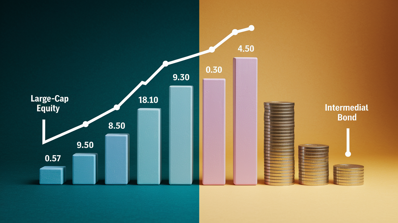
Consider a large-cap equity fund that returned 9.5 percent annually over the past five years with a standard deviation of 18 percent. During the same stretch, 3-month Treasuries averaged 2.8 percent. Subtract 2.8 from 9.5 and you’re left with 6.7 percent of excess return. Divide 6.7 by 18 and the Sharpe ratio lands around 0.37. That tells you the fund earned just over one-third of a percentage point of excess return for every percentage point of volatility. A modest payoff for the swings.
Now look at an intermediate-term bond fund that delivered 4.2 percent annualized with a standard deviation of 3.5 percent. Using the same 2.8 percent risk-free benchmark, subtract to get 1.4 percent excess return. Divide 1.4 by 3.5 and the Sharpe ratio comes in near 0.40. The bond fund’s raw return is far lower, but its smoother ride yields a risk-adjusted result that slightly edges the equity fund. This is why nominal returns alone can mislead when volatility profiles differ.
| Example Fund | Return % | Volatility % | Sharpe Ratio |
|---|---|---|---|
| Large-Cap Equity | 9.5 | 18.0 | 0.37 |
| Intermediate Bond | 4.2 | 3.5 | 0.40 |
How to Interpret Sharpe Ratios for Portfolio Decisions
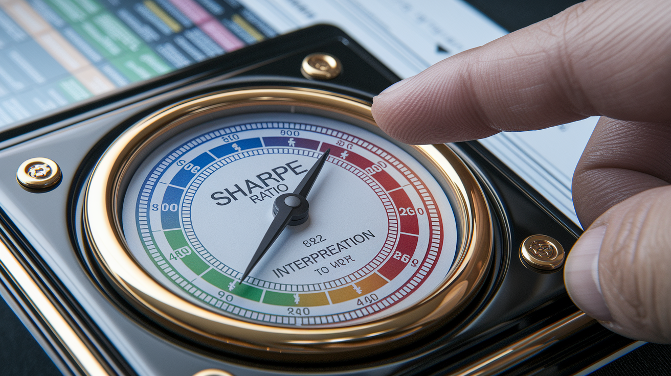
A higher number signals stronger risk-adjusted performance, but the scale isn’t intuitive at first glance. Most people rely on informal thresholds to judge whether a fund’s ratio passes muster. Context matters. Equity funds operating during calm markets may show ratios above 1.0, while the same strategies in choppy years can dip below zero if returns fail to beat the risk-free rate.
Comparisons work best when you hold the time period and fund category constant. A technology fund’s three-year Sharpe ratio of 0.85 looks weak next to a diversified equity fund’s 1.10 over the same window. Comparing a bond fund’s five-year ratio to a stock fund’s one-year figure mixes things that don’t belong together. Always align measurement horizons and asset classes before drawing conclusions.
Negative Sharpe ratios appear when a fund underperforms the risk-free rate. A reading of –0.20 means the portfolio lost ground relative to holding Treasuries, and volatility only deepened the damage. Zero suggests returns exactly matched the risk-free benchmark, offering no reward for the uncertainty.
Typical interpretation thresholds:
- Below 1.0: Considered modest or poor. Returns may not compensate adequately for volatility.
- Around 1.0: Acceptable. The fund delivers one percentage point of excess return per unit of risk.
- Above 2.0: Very good. Strong risk-adjusted performance.
- Above 3.0: Excellent. Rare outside of exceptional managers or favorable market conditions.
Limitations and Common Misunderstandings

The Sharpe ratio assumes returns follow a normal bell curve, spreading symmetrically around the average. Many fund strategies produce skewed distributions with fat tails, especially those using options, leverage, or concentrated bets. A hedge fund that posts small steady gains most months but suffers rare blowups will show a deceptively attractive Sharpe until the tail event hits. Standard deviation treats a 5 percent upside surprise the same as a 5 percent loss, even though investors care far more about the downside.
Leverage inflates the ratio artificially. A manager who borrows to double a portfolio’s position will roughly double both return and volatility, leaving the Sharpe ratio unchanged in theory. In practice, borrowing costs and margin calls introduce risks that standard deviation ignores. Two funds with identical Sharpe figures can carry vastly different leverage profiles, and the unlevered version is usually safer.
Backward-looking data can’t predict future performance. A fund’s stellar three-year Sharpe might have captured a bull run that won’t repeat. Market regimes shift, interest rates move, and manager turnover happens. Relying solely on historical ratios to choose funds locks you into yesterday’s conditions. Combine the metric with forward-looking factors like fee structure, diversification, and strategy durability.
Comparison to Other Risk-Adjusted Metrics

Sortino Ratio
The Sortino ratio swaps total volatility for downside deviation, counting only returns that fall below a chosen threshold, often zero or the risk-free rate. This tweak better reflects investor psychology. No one minds upside surprises. A fund with frequent small gains and occasional large losses will look worse under Sortino than under Sharpe, because Sortino isolates the painful swings. Use the Sortino ratio when evaluating portfolios held by risk-averse clients or when skewed return patterns make standard deviation misleading.
Treynor Ratio
Treynor replaces total volatility with beta, which measures sensitivity to broad market moves. The formula becomes (Portfolio Return – Risk-Free Rate) / Beta. This metric suits well-diversified portfolios where unsystematic risk has been eliminated through breadth. A fund with a beta of 1.2 and a Treynor ratio of 6 percent tells you it generated 6 percentage points of excess return for each unit of market risk. Compare Treynor ratios when you want to strip out the noise of stock-specific bets and focus on systematic exposure.
Information Ratio
The information ratio divides a fund’s excess return over a benchmark by the tracking error, the standard deviation of those active returns. It answers a different question. How much value did the manager add per unit of deviation from the index? A large-cap fund that hugs the S&P 500 might show a high Sharpe ratio simply by riding the market, but a low information ratio reveals minimal skill. Use this metric to evaluate active managers, pairing it with the Sharpe ratio to see both total risk-adjusted performance and benchmark-relative skill.
Final Words
You learned how the Sharpe ratio measures risk‑adjusted return, the simple formula, and the key inputs (risk‑free rate, excess return, volatility). The post walked through a five-step calculation, two fund examples, how to read the numbers, common limits, and comparisons with other metrics.
Next steps: gather consistent return data, match return periods to volatility, and compare similar funds. Don’t chase the highest number; use it as one tool.
Use the sharpe ratio explained for fund portfolios to make clearer choices about risk and return, and keep building your plan with steady, small steps.
FAQ
Q: What is the Sharpe ratio and how is it calculated?
A: The Sharpe ratio measures a portfolio’s risk‑adjusted return, calculated as (portfolio return minus risk‑free rate) divided by return standard deviation, with higher values showing better reward per unit of risk.
Q: Why does the Sharpe ratio matter for evaluating funds?
A: The Sharpe ratio matters because it shows how much return you get per unit of total risk, helping compare funds on risk‑adjusted performance instead of raw returns alone.
Q: What inputs make up the Sharpe ratio and why do they matter?
A: The inputs are the risk‑free rate, the portfolio’s excess return (over that rate), and return volatility (standard deviation); they matter because they define the baseline, reward, and risk in the ratio.
Q: How do I calculate the Sharpe ratio step-by-step?
A: To calculate, gather consistent periodic returns, choose a matching risk‑free rate, compute excess returns, calculate their standard deviation, then divide average excess return by that standard deviation.
Q: What is a good Sharpe ratio to aim for?
A: A good Sharpe ratio is above 1; above 2 is very good; above 3 is excellent. Always compare ratios using the same time frame and peer group for fairness.
Q: Can I compare Sharpe ratios between equity and bond funds?
A: You can compare Sharpe ratios between equity and bond funds, but only with the same time periods and categories—equities usually have higher volatility, so context and peers matter.
Q: What are the main limitations of the Sharpe ratio?
A: The Sharpe ratio’s limits include assuming normally distributed returns, being backward‑looking, being distorted by leverage or illiquidity, and not separating upside from downside risk.
Q: How does the Sharpe ratio compare to Sortino, Treynor, and Information ratios?
A: The Sharpe ratio uses total volatility; the Sortino ratio uses downside volatility; Treynor relates return to beta (market risk); Information ratio measures active return versus tracking error.
Q: How often should I use monthly vs annual returns when calculating the Sharpe ratio?
A: You should match return frequency and standard deviation: use monthly returns with monthly volatility or annual returns with annual volatility, then annualize if you need a different reporting period.
Q: Can you provide a simple numeric Sharpe ratio example?
A: A simple example: portfolio return 8%, risk‑free 2%, standard deviation 10% gives Sharpe = (8 − 2) / 10 = 0.6, showing modest risk‑adjusted performance.